Inner Join: From Relational Algebra to SQL Production Queries

In our previous article, we thoroughly dissected how CROSS JOIN operates as a “blind multiplication” within the database universe. Disregarding any logical alignment or inter-table relationships, it blindly ingests all rows to produce a pure Cartesian Product. However, in real-world scenarios, we cannot simply allow data to pair up at random. This is where the Inner Join family steps in as an elegant antithesis—a smart filtering operation ensuring that each row only meets its legitimate counterpart based on the rules we define.

Unfortunately, in day-to-day software engineering practices, many developers view the Inner Join as nothing more than a routine task of finding matching data using the ON keyword. Yet, if we dive deeper behind the scenes, this operation boasts a vast and rich family lineage. Its spectrum spans wide—from the Theta Join, which serves as the theoretical foundation in academia, to the Semi-Join, a go-to weapon for data engineers optimizing query performance in modern Big Data environments. Understanding the Inner Join merely on a surface level is often the root cause of subtle bugs and severe server degradation in production environments.

The primary objective of this article is to radically dissect the anatomy of the Inner Join family tree. We will not only look at it from a practical standpoint through modern SQL syntax, but also trace its logical roots academically via relational algebra expressions. By bridging formal theory and real-world database engine implementation, you will be guided to understand not just how to write a join query that successfully extracts data, but how the engine works under the hood to execute it safely, precisely, and efficiently.

2. The Conceptual Bridge: Inner Join is a “Reformed” Cross Join

To truly appreciate the power of the Inner Join family, we must first uncover one of the most fundamental secrets in database architecture: genetically, the Inner Join was never born as a standalone operator. It is the direct offspring of a CROSS JOIN that has been “reformed” and given logical guidance. In the academic realm of Relational Algebra, this phenomenon is captured with absolute elegance. The Theta Join (⨝), which serves as the blueprint for all inner operations, is defined as a Selection operation (σ) executed directly on top of a Cartesian Product (⨉). Mathematically, this lineage is locked into an absolute formula:

R ⨝_θ S ≡ σ_θ (R ⨉ S)

The formula above is not just a collection of dead symbols; it is a conceptual workflow. It dictates that to perform an Inner Join, the logical universe of the database will first roll out the CROSS JOIN carpet to generate every possible combination of data pairs between relations. Only then does it strictly curate the results through a selection operation to discard all pairs that fail to meet the (θ) condition.

Historical proof of this lineage can be easily traced back to the old-school SQL syntax of the SQL-89 standard era, often referred to as the Implicit Join. Before the INNER JOIN ... ON keywords were officially formalized, database engineers wrote join queries in a highly literal manner:

sql

-- Implicit Join Syntax (SQL-89)
SELECT *
FROM Employee E, Branch B     -- Step 1: Perform a CROSS JOIN / Cartesian Product
WHERE E.BranchId = B.BranchId; -- Step 2: Filter using Selection (Join Condition)

When you place a comma between two tables in the FROM clause, you are explicitly commanding the database to execute a CROSS JOIN. And when you append the WHERE clause, that is precisely where the selection operation takes place. The final output of the implicit query above is 100% identical to the modern INNER JOIN ... ON syntax we use today.

However, this is where the magic of modern computing comes into play. If a database engine were to execute that query literally according to its theoretical sequence—where a table with one million rows is multiplied by another one-million-row table—the server would instantly crash from an Out of Memory (OOM) error, forced to hold a trillion rows of junk combinations in memory.

This is the exact moment where the Query Optimizer steps in as the unsung hero. Modern database engines are smart enough to immediately recognize this “Cross Join + Selection” pattern. Instead of executing a blind multiplication first, the Optimizer directly translates that logic into a far more tactical physical algorithm inside the memory, such as a Hash Join or a Merge Join. Theory teaches us the logic, but the database engine executes it with efficiency.

3. Anatomy & Lineage of the Inner Join Family (Theory vs. Practice)

Now that we understand its genetic roots, let us dissect the actual tree of the vast Inner Join family. To provide a concrete and practical look, all the join variations below will be tested using a corporate retail system scenario with two primary tables:

Employee (EmployeeId, Name, Salary, BranchId)
Branch (BranchId, BranchName, CityId, MinSalaryTarget).

Below is the complete SQL script for SQL Server (T-SQL) that you can readily copy and run.

This script includes database creation, table provisioning with proper Primary Keys and Foreign Keys, as well as sample data ingestion specifically designed so that all join scenarios (Theta, Equi, Natural, down to Semi-Join) produce varied and meaningful data during your testing.

sql

-- 1. CREATE A NEW DATABASE
CREATE DATABASE CorporateRetailDb;
GO

-- Switch to the newly created database
USE CorporateRetailDb;
GO

-- 2. CREATE THE BRANCH TABLE
-- Created first because it is referenced by the Employee table
CREATE TABLE Branch (
   BranchId SMALLINT PRIMARY KEY,
   BranchName VARCHAR(30) NOT NULL,
   CityId VARCHAR(10) NOT NULL, -- Example: 'JKT', 'BDG'
   MinSalaryTarget DECIMAL(10, 0) NOT NULL
);
GO

-- 3. CREATE THE EMPLOYEE TABLE
CREATE TABLE Employee (
   EmployeeId INT PRIMARY KEY,
   Name VARCHAR(20) NOT NULL,
   Salary DECIMAL(10, 0) NOT NULL,
   BranchId SMALLINT, -- Allows NULL (for unassigned employees)
   CONSTRAINT FkEmployeeBranch
      FOREIGN KEY (BranchId) 
      REFERENCES Branch(BranchId)
);
GO

-- 4. DATA INGESTION (INSERT INTO)
-- Populate the Branch Table
INSERT INTO Branch VALUES
(10, 'Jakarta Pusat', 'JKT', 6000000),
(20, 'Jakarta Selatan', 'JKT', 6000000),
(30, 'Bandung Merdeka', 'BDG', 5500000),
(40, 'Surabaya Kota', 'SBY', 5300000),
(50, 'Ambon', 'AMB', 5000000);
GO

-- Populate the Employee Table
INSERT INTO Employee VALUES
(101, 'Budi Santoso', 6000000, 10),
(102, 'Siti Rahma',   5000000, 10),
(103, 'Andi Wijaya',  7000000, 20),
(104, 'Dewi Lestari', 4800000, 30),
(105, 'Rian Hidayat', 5200000, 40),
(106, 'Staf Magang',  3000000, NULL);
GO

Here is a comprehensive breakdown of each member of the Inner Join family:

A. Theta Join (θ-join)

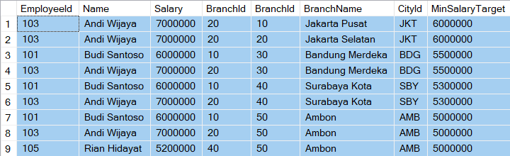
The Concept: A Theta Join is the most generic form of an inner join. The symbol θ (Theta) represents any general mathematical comparison operator, such as <, >, ≤, ≥, or ≠. Therefore, the relationship between tables does not always have to be locked by an “equals” sign.
Real-World Case: The company wants to perform a cross-analysis of macro performance. You are tasked with pairing every single employee with any branch that has a MinSalaryTarget lower than that employee’s salary—regardless of whether the employee actually works at that branch or not.
Relational Algebra Expression:

Employee ⨝_{Employee.Salary> BranchMinSalaryTarget} Branch

SQL Query:

SELECT *
FROM Employee E
INNER JOIN Branch B
ON E.Salary > B.MinSalaryTarget;

Execution Result:

B. Equi-Join

The Concept: An Equi-Join is a direct derivative or a specific case of the Theta Join. The only difference is that the (θ) operator is strictly locked and limited exclusively to the equality operator (=). This is the most common type of join encountered in day-to-day application development.
Real-World Case: Management requests a standard operational report to map staff data. Your task is to pair each employee’s name with the branch where they are explicitly deployed, based on matching branch IDs in both tables.
Relational Algebra Expression:

Employee ⨝_{Employee.BranchId=Branch.BranchId} Branch

SQL Query:

SELECT *
FROM Employee E
INNER JOIN Branch B
ON E.BranchId = B.BranchId;

Execution Result:

C. Natural Join

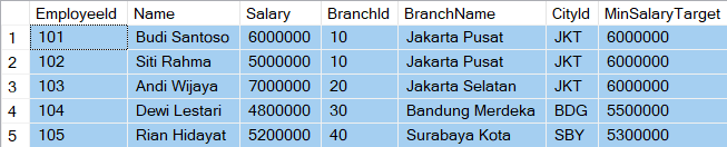
The Concept: A Natural Join goes one step further in practicality than an Equi-Join. It is a join operation that works automatically behind the scenes without requiring an explicit condition definition (ON). The database engine scans both tables, detects columns that share the exact same name and data type (which in our case is BranchId), and uses them as the bridge for an Equi-Join. Its defining unique feature is that it automatically merges duplicate columns, meaning the linking column appears only once in the final result.
Real-World Case: You want to write a query for a staff-and-branch relationship report using the shortest syntax possible, while ensuring that the extracted data (SELECT *) is clean of redundant, twin BranchId columns that clutter the view.
Relational Algebra Expression: Written purely using the join symbol without any subscript because its mechanism is implicit.

Employee ⨝ Branch

SQL Query:

-- Valid on supporting DBMSs
-- such as PostgreSQL, MySQL, Oracle
SELECT *
FROM Employee
NATURAL JOIN Branch;

-- For non-supporting DBMSs
-- such as SQL Server, DB2
SELECT E.*, BranchName,
   CityId, MinSalaryTarget
FROM Employee E
INNER JOIN Branch B
ON E.BranchId = B.BranchId

-- or
SELECT EmployeeId,
   Name, Salary, B.*
FROM Employee E
INNER JOIN Branch B
ON E.BranchId = B.BranchId

Execution Result:

D. Left Semi Join & Right Semi Join

Left Semi Join

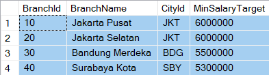
The Concept: Why is the Semi-Join classified under the broad Inner Join family? The answer lies in its behavior: it only passes data that has a match between both tables. However, there is a fundamental difference compared to conventional joins. It exclusively returns columns from only one side of the tables.
Real-World Case: You are asked to build a dropdown menu feature for an internal application that only displays a list of Branches that currently have active employees. If there is a new branch that does not have any staff yet, that branch must not appear. You do not need any detailed employee data; you simply need to verify their existence within that branch without causing duplicate branch rows.
Relational Algebra Expression:

Branch ⋉ Employee

SQL Query:

-- Use DISTINCT to 
-- prevent duplication
SELECT DISTINCT B.*
FROM Branch B 
INNER JOIN Employee E
ON B.BranchId = E.BranchId;

Execution Result:

Right Semi Join

A Left Semi-Join query between R and S will produce the exact same data as a Right Semi-Join between S and R.

R ⋉ S ≡ S ⋊ R

Both expressions share the exact same meaning: Retrieve all columns from table R that have a matching pair in table S. Therefore, the previous Left Semi-Join case could also be written using a Right Semi-Join:

Employee ⋊ Branch

SQL Query:

SELECT DISTINCT B.*
FROM Employee E
INNER JOIN Branch B 
ON E.BranchId = B.BranchId;

4. DBMS Reality: Why Natural Join & USING Are Treated as Second-Class Citizens?

When we step out of the academic classroom and into the reality of the industry, we encounter an interesting landscape. Not every feature formalized in the official ANSI SQL standards is embraced with open arms by the giants of the Database Management System (DBMS) world. NATURAL JOIN and the USING clause are prime examples of standard features with a tragic fate: highly praised in some environments, yet treated as second-class citizens—or outright rejected—in others.

Engine Support Map

If we map out the modern database ecosystem, we can see a clear ideological divide regarding the adoption of these features:

The Supporting Camp (Oracle, PostgreSQL, MySQL, MariaDB, SQLite): DBMSs in this group strictly adhere to ANSI SQL standards. They provide full support for NATURAL JOIN along with all its combination variants (such as NATURAL LEFT JOIN), while also supporting the USING clause.
The Rejecting Camp (Microsoft SQL Server, IBM Db2): If you attempt to write a NATURAL JOIN statement or a USING clause inside Microsoft SQL Server, the system will instantly stall and throw an error message: “Incorrect syntax near the keyword…”. SQL Server has consciously and stubbornly rejected the presence of both syntaxes since the day they were conceived.

The Code Safety Debate: Unveiling The “Implicit” Risk

Why are giants like Microsoft SQL Server or IBM Db2 reluctant to implement a feature that could otherwise make code more concise? The answer is not rooted in technological limitations, but rather in an architectural decision to preserve long-term code safety and stability.

NATURAL JOIN operates on an implicit principle—it is a black box. It guesses which columns to link solely based on matching names. This implicit nature hides a latent danger in production environments.

Imagine you have an operational query that has been running safely for years in your application:

SQL

-- Runs smoothly because initially, 
-- only the 'BranchId' column shares the same name
SELECT *
FROM Employee
NATURAL JOIN Branch;

One day, a Database Administrator (DBA) performs routine maintenance. For performance auditing and system tracking needs, the DBA adds two new columns: Status (for active status) and CreatedAt (for the data recording timestamp) to both the Employee and Branch tables.

At that exact second, your NATURAL JOIN query will quietly break. The database engine, blindly following the “natural” principle, will automatically alter its internal join logic. It no longer just matches BranchId. Instead, it is now forced to also match Employee.Status = Branch.Status AND Employee.CreatedAt = Branch.CreatedAt. As a result, a query that used to display thousands of rows suddenly returns zero rows—completely empty—without throwing a single error or warning to your application system. A feature originally intended to shorten code transforms into a ticking time bomb, waiting to explode the moment the database schema evolves.

The Middle-Ground Solution: The USING Clause

Aware of the fatal risks posed by the “guessing game” nature of NATURAL JOIN, the ANSI SQL standard formulated a much more elegant middle-ground solution: the USING clause.

The USING clause marries the concise output of a Natural Join with the safety of an Explicit Join. Here, you do not let the database guess; instead, you explicitly lock in the name of the column that serves as the bridge. Yet, you still retain the privilege of having duplicate twin columns automatically cleaned up and merged in the extracted data.

SQL

-- Explicitly specifies the column;
-- Supported by Postgres, Oracle, and MySQL
SELECT *
FROM Employee
INNER JOIN Branch
USING (BranchId);

With the syntax above, if a DBA adds the Status or CreatedAt columns to both tables in the future, your query is guaranteed to remain 100% safe because the relationship between the tables has been locked tightly to the BranchId column alone. Furthermore, thanks to the rules of the USING clause, the result of SELECT * will not display dual BranchId columns side-by-side. Instead, it merges them into a single, clean column at the very beginning of the result table.

Unfortunately, for those of you building application architectures on top of Microsoft SQL Server, this middle-ground solution remains unavailable. You must always stay faithful to the conventional ON E.BranchId = B.BranchId clause to guarantee code portability and security.

5. The Semi-Join Logical Battle: INNER JOIN vs. IN vs. EXISTS

In large-scale application development, efficiency is no longer an option—it is a necessity. One of the fiercest battles in query optimization occurs when we want to perform a Semi-Join operation—filtering data in one table based on the existence of matching data in another.

Functionally, there are three popular ways developers achieve this result: using an INNER JOIN, the IN clause, or the EXISTS clause. While all three can yield identical data, their underlying mechanics under the hood dictate whether your server will run smoothly or suddenly grind to a halt.

Why Using INNER JOIN (Then Projecting) Is Bad Practice

One of the most common computational sins committed by developers is forcing an INNER JOIN to act as a filter, and then cutting down its columns using projection (SELECT TableA.*). In terms of the final output, this trick might seem successful. Architecturally, however, it is a memory disaster known as the Multiplying Rows effect.

An INNER JOIN is designed to bridge and combine rows. If a single row in the left table matches ten rows in the right table (a one-to-many relationship), the INNER JOIN will duplicate that left-table row ten times inside the memory. Performing a SELECT E.* (from Employee) will not erase the fact that the database engine has already wasted CPU and I/O resources to duplicate those rows, only for you to force it to discard the right-table columns right afterward.

The Analogy of the Teacher and Remedial Students: Imagine the principal asks you to gather data: “Which teachers have remedial students in their classes?”
The INNER JOIN Approach: You approach each teacher and pair their name with every single student of theirs who needs remediation. If Teacher A has 30 remedial students, you will write Teacher A’s name 30 times on your paper. In the end, since you only need the list of teachers, you are forced to painstakingly eliminate the 29 duplicate entries using a exhausting process (DISTINCT). This is a massive waste of energy.

The “Booby Trap” of the IN Clause

Seeing the flaws of the INNER JOIN mentioned above, many developers turn to the IN clause because its query syntax is much cleaner and more intuitive:

sql

SELECT *
FROM Branch
WHERE BranchId IN
  (SELECT BranchId
   FROM Employee);

Logically, this query works well and is free from row duplication issues. However, the IN clause conceals a critical “booby trap” regarding NULL values. In the SQL universe, comparisons with NULL utilize three-valued logic (True, False, Unknown). The operation BranchId = NULL will never evaluate to True or False; it evaluates to Unknown.

In a standard Semi-Join operation, a NULL value within the subquery might simply be passively ignored. However, a genuinely horrific danger arises when you flip this logic into an Anti-Join using NOT IN:

sql

-- DO NOT DO THIS if the 
-- Employee.BranchId table contains NULL values!
SELECT *
FROM Branch
WHERE BranchId NOT IN
  (SELECT BranchId
   FROM Employee);

If the Employee table contains even a single row where the BranchId column is NULL, the NOT IN query above will automatically return completely empty (0 rows) forever! The database engine translates NOT IN as a strict chain of AND operations (e.g., BranchId != 10 AND BranchId != 20 AND BranchId != NULL). Because that final comparison evaluates to Unknown, the entire chain of WHERE conditions is instantly invalidated and fails completely.

Why EXISTS is King?

To win this logical battle, the EXISTS clause stands as the undisputed king. EXISTS is designed with a Short-Circuit Filtering mechanism.

Returning to our school analogy: with EXISTS, you approach Teacher A and ask if they have any remedial students. The exact moment Teacher A points to just one remedial student, you instantly stop searching that classroom, write Teacher A’s name on the list, and immediately skip to Teacher B. The database engine does not care how many matching records exist in the right table; as soon as the first match is found, the main table row is declared qualified.

sql

SELECT *
FROM Branch B
WHERE EXISTS
  (SELECT 1
   FROM Employee E
   WHERE E.BranchId = B.BranchId);

The absolute advantages of EXISTS include:

Immune to NULL Values: The EXISTS clause does not utilize direct value comparisons on the subquery elements; instead, it purely evaluates the existence of rows (True or False). The presence of NULL data inside the table will never break your query filter logic.
Query Optimizer Intelligence: In modern RDBMSs, when you write an EXISTS syntax, the Query Optimizer immediately recognizes your specific intent. The engine will not repeatedly execute the subquery for every single row. Instead, it translates it under the hood into a physical index-based Left Semi-Join (Index Seek) that is incredibly fast and memory-efficient.

6. Conclusion & Best Practices

Our journey dissecting the lineage of the Inner Join family leads us to one vital conclusion: writing SQL queries in a professional environment is not just about the art of “as long as the data comes out.” Joining two or more tables is a matter of logical precision, efficient memory allocation, and ensuring long-term immunity against dynamic database schema changes.

As a wise developer or data analyst, here is a summary of practical guidelines (best practices) that you can bring into your next real-world project:

Understand Data Characteristics (Cardinality): Before settling on a specific type of join, make sure you know whether the relationship between the two tables is one-to-one, one-to-many, or many-to-many. Misanalyzing this relationship is the root cause of row counts exploding in memory.
Choose EXISTS for Semi-Join Operations: Drop the habit of using nested INNER JOINs or IN clauses if your pure objective is to filter for data existence. The EXISTS clause is the best “ninja way”—immune to NULL value traps while remaining highly friendly to the Query Optimizer.
Prioritize Code Clarity (Explicit Join): Avoid using NATURAL JOIN in production environments. Writing out conditions explicitly using the ON clause (or USING on supporting DBMSs) will save your system from silent, undetected mass failures when table column structures are modified in the future.
Maintain Data Type Consistency: Ensure that the columns you use as a join bridge share the exact same data type to avoid implicit conversions, which can kill database index functionality.

Let’s Discuss!

How about you? Have you ever been trapped in a production “horror story” due to choosing the wrong type of join, or been caught off guard by a mysterious NULL value? Which DBMS do you currently use most often to optimize complex queries?

Let’s share your experiences, critiques, or questions in the comment section below! If this article provided a new perspective and proved beneficial to your learning journey, feel free to share it with your fellow developers.

See you in the next article! We will step across the INNER JOIN boundary to thoroughly uncover the darkness and mysteries often hidden by OUTER JOINs (Left, Right, and Full Outer Join).

References

Codd, E.F. (March 1972). “Relational Completeness of Data Base Sublanguages” in Computer Sciences. San Jose, California: IBM Research Laboratory.

Connolly, Thomas M., & Begg, Carolyn E. (2015). Database Systems: A Practical Approach to Design, Implementation, and Management. 6th Edition. Essex, England: Pearson Education.

Coronel, C., Steven, M., Crockett, K., & Blewett, C. (2020). Database Principles: Fundamentals of Design, Implementation, and Management. 3rd Edition. Hampshire, United Kingdom: Cengage Learning

1. Introduction